


A mapping and positioning method for vehicle Lidar based on vision and IMU
In order to solve the problem of non-uniform motion distortion of LiDAR, a three-dimensional map simultaneous localization and mapping (SLAM) method is constructed by combining visual inertia odometer and lidar odometer. The pre-processed timestamp alignment data is initialized by visual estimation and pre-integration of IMU. By constrained sliding window optimization and high frequency pose of visual odometer, the traditional radar uniform motion model is improved to a multistage uniform acceleration model. Thus reducing point cloud distortion. At the same time, the Levenberg ~ Marquard LM method is used to optimize the laser odometer, and a loop detection method combining the word bag model is proposed. Finally, a three-dimensional map is constructed. Based on the real vehicle test data, the mean error and median error are increased by 16% and 23% respectively compared with the results of LEGO ̄LOAM(Light and ground optimization LiDAR range measurement and variable terrain map ping) method.
0 Introduction
With the release of the "Intelligent Vehicle Innovation Development Strategy" in February 2020, the research of automotive driverless technology has become a hot topic in universities and industry. Simultaneous localization and mapping SLAM technology is an important part of driverless technology. When the unmanned vehicle fails in the global positioning system GPS, SLAM technology can independently estimate and navigate the unmanned vehicle's attitude by relying on its own sensors without prior information [1]. At present, mainstream SLAM methods can be divided into camera-based visual SLAM and radar-based laser SLAM according to sensor types [2]. In recent years, the integration of inertial measurement units (IMU visual SLAM) has gradually become a research hotspot in this field due to the advantages that absolute scale can be estimated and the image quality is not affected by IMU visual SLAM [3].
Visual SLAM can be further divided into feature point method and optical flow method. The feature point method tracks the feature points through the feature point matching. Finally, the reprojection optical flow rule is based on the constant gray level assumption, and the matching between the descriptor and the feature point in the feature point method is replaced by the optical flow tracking. Among the SLAM schemes of eigenpoint method, ORB ̄SLAM(directional FAST and rotating BRIEF) is the most representative. ORB has the invariance of viewpoint and illumination, and the extraction of key frames and deletion of redundant frames also ensure the efficiency and accuracy of BA(bundle adjustment) optimization [4-5]. Considering that pure visual SLAM is prone to frame loss during rotation, especially because pure rotation is sensitive to noise, Xu Kuan et al. [6] integrated IMU and vision, optimized the pre-integrated IMU information and visual information by using Gauss-Newton method, and optimized the visual reprojection error and IMU residual by using graph optimization method. To obtain a more accurate pose. VINS ~ MONO(a robust universal monocular visual inertia state estimator) is outstanding in outdoor performance, which uses IMU+ monocular camera scheme to restore the scale of the target. Because of the use of optical flow tracking as the front end, ORB ̄SLAM is more robust than using descriptors as the front end, and ORB ̄SLAM is not easy to lose track when moving at high speed [7].
However, pure visual SLAM requires moderate lighting conditions and distinct image features, making it difficult to build 3D maps outdoors. SLAM can build outdoor 3D maps, but it is easy to produce uneven motion distortion in the process of motion, and inaccurate positioning in degraded scenes. Therefore, based on the point cloud information collected by LiDAR, a multi-sensor integrated outdoor 3D map construction and location method is proposed in this paper. The method first computes the visual inertial odometer VIO and outputs the high frequency pose. Then the motion distortion of the LIDAR is removed by high frequency pose using the laser ranging technology ꎬLO(ꎬ), and the 3D map is constructed.
1 Algorithm framework
The algorithm framework is roughly divided into two modules: visual inertia odometer module, laser odometer module and mapping module. The visual inertia odometer uses KLT(kanade-lucas-tomasi tracking) optical flow to track the two adjacent frames, and uses IMU pre-integration as a predictive value of the motion of the two adjacent frames. In the initialization module, vision and IMU pre-integral are loosely coupled, solving for gyroscope bias, scale factor, gravity direction, and velocity between adjacent frames. The residuals based on visual construction and IMU construction are optimized by sliding window method. Output the HF absolute pose calculated by the VIO. The external parameter matrix is obtained by the joint calibration of the camera radar between the two modules, and the absolute pose in the camera coordinate system is converted to the radar coordinate system.
The laser odometer and mapping module divide the point cloud into different types of cluster points to facilitate subsequent feature extraction, and then fuse the high-frequency VIO pose to improve the traditional radar uniform motion model into a multistage uniform acceleration model. At this point, the point cloud combines information from the camera and the IMU. By ICP(it ̄ r-nearest point) matching, LM is used to optimize the pose transformation matrix between two frame point clouds and convert it to the initial point cloud coordinate system. Finally, combined with the cyclic detection based on the bag of words model, the three-dimensional map is constructed.
2 Drawing and positioning methods
2.1 Camera and IMU data preprocessing
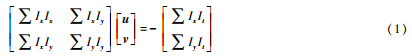
Due to the high feature extraction efficiency of FAST, KLT optical flow tracking does not require description, so both are selected for feature extraction and optical flow tracking. Let Ix and Iy respectively represent the image gradient of pixel brightness in the x and y directions, represent the time gradient u and v in the t direction, and represent the velocity vector of optical flow on the x and y axes respectively. According to the KLT optical flow principle, the constraint equation is constructed, and the equations of u and v are obtained by the least square method:
In each new image, KLT algorithm is used to track the existing feature points and detect the new feature points. In order to ensure the uniform distribution of feature points, the image is divided into 18×10 sub-regions with the same size, each sub-region can extract up to 10 FAST corner points, and each image can maintain 50 ~ 200 FAST corner points. In outdoor scenes, the displacement between two adjacent frames is large, and the brightness value of each pixel may change suddenly, which has a bad effect on the tracking of feature points. Therefore, it is necessary to remove the outliers of the feature points and then project them onto the unit sphere. Outliers are eliminated using RANSAC algorithm combined with Kalman filter to achieve more robust optical flow tracking in outdoor dynamic scenes. Figure 2 shows the feature point tracking of outdoor scenes without and with RANSAC algorithm. As can be seen, the use of RANSAC algorithm reduces the case of mistracking.
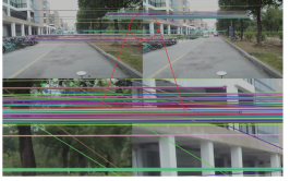
(a) No RANSAC algorithm is used for feature point tracking
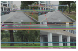
(b) Feature point tracking using RANSAC algorithm
Figure 2 Influence of RANSAC algorithm on feature point tracking
IMU responds quickly, is not affected by imaging quality, and can estimate the absolute scale feature complement of visual positioning of non-structured objects on outdoor surfaces. During camera attitude estimation, if all poses corresponding to all sampling times of IMU are inserted between frames for optimization, program operation efficiency will be reduced [8-9], and pre-integration processing of IMU is required to convert the measured values of acceleration and angular velocity of high-frequency output into a single observed value. The measured value is linearized again in nonlinear iteration to form a constraint factor of the inter-frame state quantity [7]. The continuous time IMU pre-integration is shown in the following equation.
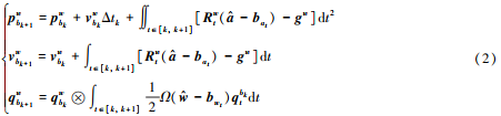
Where :b is the IMU coordinate system, w is the origin of the coordinate system where the IMU is located during initialization, that is, the world coordinate system at and wt are the acceleration and angular velocity measured by the IMU, qb t k is the rotation from the IMU coordinate system to the world coordinate system at the time, and Ω is the quaternion right multiplication. Integrate all IMU data between frame k and frame k+1. The position (P), speed (v), and rotation (Q) of the k+1 frame are obtained. This PvQ is used as the initial value of the visual estimate, where the rotation is in quaternion form.
2.2 Sliding window optimization
Initialization module to restore the scale of monocular camera, visual information and IMU information need to be loosely coupled. Firstly, SFM is used to solve the pose of all frames and the 3D position of all signposts in the sliding window, and then align them with the pre-integral value of IMU, so as to solve the angular velocity bias, gravity direction, scale factor and the velocity corresponding to each frame. With the operation of the system, the number of state variables increases, and the sliding window method [10] is used to optimize the state variables in the window. The optimization vector xi defined in the i moment window is as follows.

Where, Ri pi is the rotation and displacement of the camera pose and vi is the speed abi of the camera in the world coordinate system, and ωbi is the acceleration bias and angular velocity bias of IMU respectively.
The set of all xi for all frames participating in the optimization slide window at time k is Zk for all observations of the Xk system. Combined with Bayes formula, the maximum posterior probability is used to estimate the state quantity of the system, as follows:

The maximum a posteriori problem is transformed into an optimization problem, and the optimization objective function is defined in the following equation.

Where X * k is the maximum estimated posterior value, r0 is the initial sliding window residual, and rIij is the IMU observation residual. The proposed calibration method jointly calibrates the camera and the LiDAR to determine the relative attitude of the camera and the radar. The optimized VIO attitude is converted into a radar coordinate system and then output to the laser odometer module. At the same time, the word package DBoW2 constructed by the BRIEF descriptor is used to calculate the similarity of the current frame and for loop detection.
2.3 Point cloud data preprocessing
The LEGO_LOAM scheme is improved in the point cloud preprocessing part, and the point cloud is divided into ground points, effective clustering points and outliers, which are divided into two steps:
1) Ground point cloud extraction can divide the point cloud into 0.5m × 0.5m grids, calculate the height difference between the highest point and the lowest point in the grids, and classify the grids whose height difference is less than 0.15m as ground points.
2) Effective clustering point extraction. After marking ground points, perturbations of some small objects will affect the next interframe registration process. Therefore, European-style clustering is carried out for point clouds ꎬ, and the points with cluster number less than 30 or the line harness occupying less than 3 in the vertical direction are filtered out
2.4 High-frequency VIO pose removes point cloud distortion
Due to the non-uniform motion distortion of point cloud in the scanning process of mechanical lidar [13], in order to improve the accuracy of point cloud registration, high-frequency pose output by VIO is used to remove the point cloud distortion. First, align the time stamps of the two sensor systems, as shown in Figure 3. Define tLq as the time stamp of the radar at the QTH scan ꎬ and define tV-Ik as the time stamp of the VIO system at the KTH pose output ꎬ, then the time alignment stamp is realized by the following formula:
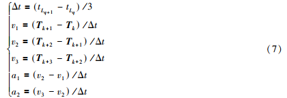
The velocity, displacement and Euler Angle of the point cloud are calculated by interpolation through the displacement and velocity of the two stages, and the distortion caused by the non-uniform motion of the radar is eliminated.
2.5 Extraction and matching of point cloud feature points
Point cloud feature points mainly include two types: plane feature points and edge feature points. As shown in Figure 4, due to the larger curvature of the breakpoint and the smaller curvature of the parallel points, they will be mistaken as edge points and plane points respectively [14]. Therefore, before feature extraction, it is necessary to remove the breakpoints on the section and the parallel points parallel to the direction of the laser line. The roughness of the point cloud is defined as the set of the five points closest to the point cloud at time k. Threshold segmentation of edge points and surface points is carried out by the size of ckꎬ i, as follows:

3 Verify the actual scenario
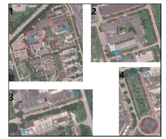
FIG. 5 Experimental route
The method in this paper was marked as A method and LEGO ̄LOAM method as B method. Table 1 shows the comparison between method A and method B, both of which are true values, i.e. GPS data for comparison. In Table 1, Max is the maximum error, Mean is the average error, mean is the Median error, Min is the minimum error, RMSE is the root mean square error, SSE is the square error, and STD is the standard deviation.
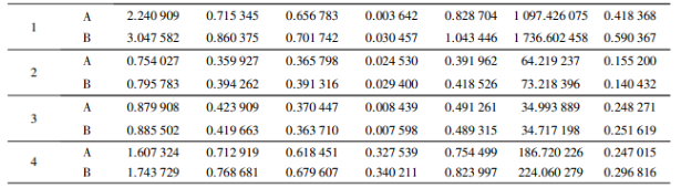
Table 1 Comparison of real vehicle verification results
It can be seen from the control group in sequence 1 to 4 in Table 1 that method A has a smaller error than method B in terms of various errors of each type of route. Under the large-scene map, the maximum error is reduced by 26%, the average error by 16%, the median error by 23%, the minimum error by 88%, the root-mean-square error by 20%, the sum of the squares by 36%, and the standard deviation by 30%. Figure 7(a) and 7(b) show the trajectory comparison and error analysis between method A and the true value under A large-scene map. Figure 7(c) and 7(d) show the trajectory comparison and error analysis between Method B and the true value under a large-scene map. Compared with method B, the errors of method A in all aspects are effectively reduced under large-scene map construction.
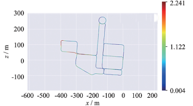
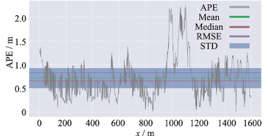
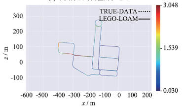
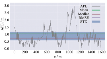
Figure 7. Error comparison between the trajectory built by the two methods and the trajectory of the true value
4 Conclusion
The point cloud non-uniform motion distortion exists in the three-dimensional construction of outdoor LiDAR. The visual inertia odometer is integrated with the traditional laser SLAM method. The uniform motion model of radar is improved to a multi-stage uniformly accelerated motion model, and the word bag model is introduced into the loop detection module. Comparing with LEGO ̄LOAM method on the absolute pose error of drawing, the average error and median error of this method are increased by 16% and 23% respectively, and the accuracy of drawing construction is greatly improved. It can be seen that the multi-stage uniformly accelerated radar motion model can effectively reduce the cumulative odometer error under long-term mapping. Compared with the traditional method, the proposed double loop detection has stronger time constraints in the loop time accuracy, and can meet the needs of outdoor 3D mapping.
References:
[1] HENING S IPPOLITO C A KRISHNAKUMAR K S et al. 3D LiDAR SLAM integration with GPS/INS for UAVs in urban areas GPS ~ degraded environments[C] / / AIAA Information Systems ~ AIAA Infotech@Aerospace. Grapevine: AIAA 2017: 0448.
[2] SHIN Y S PARK Y S KIM A. Direct visual SLAM using sparse depth for camera ̄lidar system[C] / / International Conference on Robotics and Automation (ICRA). Brisbane: IEEE 2018:1-8.
[3] NUTZI G WEISS S SCARAMUZZA D et al. Fusion of IMU and vision for absolute scale estimation in monocular SLAM[J].Journal of Intelligent & Robotic Systems201161(1/2/3/4): 287-299.
[4] MUR ̄ARTAL R MONTIEL J M M TARDOS J D ORB ̄SLAM: a versatile and accurate monocular SLAM system[J]. IEEE Transactions on Robotics 2015 31(5): 1147-1163.
[5] GAO Xiang, Zhang Tao, Liu Yi, et al. Visual SLAM Fourteen lectures: From Theory to Practice [M]. Beijing: Publishing House of Electronics Industry 2017. (Chinese)
[6] Xu Kai. Research on binocular Visual SLAM based on IMU information fusion [D]. Harbin: Harbin Institute of Technology 2018. (Chinese)
[7] QIN T LI P SHEN S. Vins ̄mono: a robust and versatile monocular visual ̄inertial state estimator[J]. IEEE Transactions on Robotics 2018 34(4): 1004-1020.
[8] INDELMAN V WILLIAMS S KAESS M et al. Factor graph based incremental smoothing in inertial navigation systems[C] / /15th International Conference on Information Fusion. Singapore: IEEEꎬ 2012:2154-2161.
[9] Cheng Chuanqi, Hao Xiangyang, Li Jiansheng, et al. Monocular vision/inertial integrated navigation algorithm based on nonlinear optimization [J]. Journal of Inertia Technology, 2017,25(5):643-649.
[10] HINZMANN T SCHNEIDER T DYMCZYK M et al. Monocular visual ̄inertial SLAM for fixed ̄wing UAVs using sliding window based nonlinear optimization[J]. Lecture Notes in Computer Science 2016 10072: 569-581.
[11] UNNIKRISHNAN R HEBERT M. Fast extrinsic calibration of a laser rangefinder to a camera: CMU ̄RI ̄ TR-05-09 [R].Pittsburgh: Robotics Institute Carnegie Mellon University 2005.
[12] KASSIR A PEYNOT T. Reliable automatic camera ̄laser calibration[C] / / Proceedings of the 2010 Australasian Conference on Robotics & Automation. Australasia: ARAA 2010: 1-10.
[13] ZHANG J SINGH S. LOAM: lidar odometry and mapping in real ̄time[C] / / Robotics: Science and Systems. Berkeley: CA 2014 2:9.
[14]SHAN T ENGLOT B. Lego ̄loam: lightweight and ground ̄optimized lidar odometry and mapping on variable terrain[C] / /
IEEE/RSJ International Conference on Intelligent Robots and Systems. Madrid: IEEEꎬ 2018: 4758-4765.